Multiple 3D scans are necessary to digitalize environments without occlusions. To create a correct and consistent model, the scans have to be merged into one coordinate system. This process is called registration. If robot carrying the 3D scanner were precisely localized, the registration could be done directly based on the robot pose. However, due to the unprecise robot sensors, self localization is erroneous, so the geometric structure of overlapping 3D scans has to be considered for registration.
The following method for registration of point sets is part of many publications, so only a short summary is given here. The complete algorithm was invented in 1992 and can be found, e.g., in [7]. The method is called Iterative Closest Points (ICP) algorithm.
Given two independently acquired sets of 3D points, ![]() (model
set,
(model
set, ![]() ) and
) and ![]() (data set,
(data set, ![]() ) which
correspond to a single shape, we aim to find the transformation
consisting of a rotation
) which
correspond to a single shape, we aim to find the transformation
consisting of a rotation ![]() and a translation
and a translation ![]() which
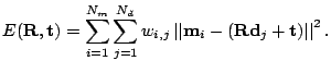
minimizes the following cost function:
which
minimizes the following cost function:
The ICP algorithm calculates iteratively the point
correspondences. In each iteration step, the algorithm selects
the closest points as correspondences and calculates the
transformation (
![]() ) for minimizing equation
(
) for minimizing equation
(![]() ). The assumption is that in the last iteration step
the point correspondences are correct. Besl et al. prove that
the method terminates in a minimum [7]. However,
this theorem does not hold in our case, since we use a maximum
tolerable distance
). The assumption is that in the last iteration step
the point correspondences are correct. Besl et al. prove that
the method terminates in a minimum [7]. However,
this theorem does not hold in our case, since we use a maximum
tolerable distance
![]() max for associating the scan
data. Such a threshold is required, given that the 3D scans
overlap only partially. Fig.
max for associating the scan
data. Such a threshold is required, given that the 3D scans
overlap only partially. Fig. ![]() (top) shows three
frames, i.e., iteration steps, of the ICP algorithm. The bottom
part shows the start poses
(top) shows three
frames, i.e., iteration steps, of the ICP algorithm. The bottom
part shows the start poses
![]() from which a correct
matching is possible, here with only three degrees of freedom.
from which a correct
matching is possible, here with only three degrees of freedom.
![\includegraphics[width=50mm]{frame1_final}](img22.png)
![\includegraphics[width=50mm]{frame2_final}](img23.png)
![\includegraphics[width=50mm]{frame3_final}](img24.png) ![\includegraphics[width=68mm,height=46mm]{gr_th__1}](img25.png)
![\includegraphics[width=65mm]{gr_th__2}](img26.png)
|