Calculating Heuristic Initial Estimations for ICP Scan Matching

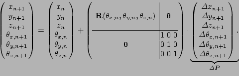
To match two 3D scans with the ICP algorithm it is necessary to have a sufficient starting guess for the second scan pose. In earlier work we used odometry [23] or the planar HAYAI scan matching algorithm [16]. However, the latter cannot be used in arbitrary environments, e.g., the one presented in Fig. 1 (bad asphalt, lawn, woodland, etc.). Since the motion models change with different grounds, odometry alone cannot be used. Here the robot pose is the 6-vector $\M {\vec P} = (x, y, z, \theta_{x}, \theta_{y}, \theta_{z})$ or, equivalently the tuple containing the rotation matrix and translation vector, written as 4$\times$4 OpenGL-style matrix $\M P$ [8]. The following heuristic computes a sufficiently good initial estimation. It is based on two ideas. First, the transformation found in the previous registration is applied to the pose estimation - this implements the assumption that the error model of the pose estimation is locally stable. Second, a pose update is calculated by matching octree representations of the scan point sets rather than the point sets themselves - this is done to speed up calculation:

1. Extrapolate the odometry readings to all six degrees of freedom using previous registration matrices. The change of the robot pose $\Delta \M P$ given the odometry information $(x_n,z_n,\theta_{y,n})$, $(x_{n+1},z_{n+1},\theta_{y,n+1})$ and the registration matrix $\M R({\theta_{x,{n}}}, {\theta_{y,{n}}}, {\theta_{z,{n}}})$ is calculated by solving:

   
   
   

   $$\left( \begin{array}{c} x_{n+1} \\ y_{n+1} \\ z_{n+1} \\ {... ...Delta {\theta_{z,{n+1}}} \\ \end{array}\right).}_{\Delta \V P}$$

   
   

   
   Therefore, calculating $\Delta \V P$ requires a matrix inversion. Finally, the 6D pose $\M P_{n+1}$ is calculated by
   
   

   $$\M P_{n+1} = \Delta \M P \cdot \M P_{n}$$

   
   using the poses' matrix representations.
   
2. Set $\Delta \V P_$best to the 6-vector $(\V t, \V R({\theta_{x,{n}}}, {\theta_{y,{n}}}, {\theta_{z,{n}}})) = (\VNull , \V R(\!\VNull ))$.
   
3. Generate an octree $\OctB _M$ for the $n$th 3D scan (model set $M$).
   
4. Generate an octree $\OctB _D$ for the $(n+1)$th 3D scan (data set $D$).
   
5. For search depth $t \in [t_$Start$,\ldots,t_$End$]$ in the octrees estimate a transformation $\Delta \V P_$best$= (\V t, \V R)$ as follows:
   1. Calculate a maximal displacement and rotation $\Delta \V P_$max depending on the search depth $t$ and currently best transformation $\Delta \V P_$best.
   2. For all discrete 6-tuples $\Delta \V P_i \in [- \Delta \V P_$max$,\Delta \V P_$max$]$ in the domain $\Delta \V P = (x,y,z,\theta_x, \theta_y,\theta_z)$ displace $\OctB _D$ by $\Delta \M P_i \cdot \Delta \M P \cdot \M P_n$. Evaluate the matching of the two octrees by counting the number of overlapping cubes and save the best transformation as $\Delta \V P_$best.
      
6. Update the scan pose using matrix multiplication, i.e.,
   

   $$\M P_{n+1} = \Delta \M P_ \cdot \Delta \M P \cdot \M P_{n}.$$

   
   

Figure 2: Left: Two 3D point clouds. Middle: Octree corresponding to the black point cloud. Right: Octree based on the blue points.

Note: Step 5b requires 6 nested loops, but the computational requirements are bounded by the coarse-to-fine strategy inherited from the octree processing. The size of the octree cubes decreases exponentially with increasing $t$. We start the algorithm with a cube size of 75 cm$^3$ and stop when the cube size falls below 10 cm$^3$. Fig. 2 shows two 3D scans and the corresponding octrees. Furthermore, note that the heuristic works best outdoors. Due to the diversity of the environment the match of octree cubes will show a significant maximum, while indoor environments with their many geometry symmetries and similarities, e.g., in a corridor, are in danger of producing many plausible matches.

After an initial starting guess is found, the range image registration from section 2 proceeds and the 3D scans are precisely matched.