Experiment and Results

**Figure 3:** 3D model of an experiment to digitize part of the campus of Schloss Birlinghoven campus (top view). Left: Registration based on odometry only. Right: Model based on incremental matching right before closing the loop, containing 62 scans each with approx. 100000 3D points. The grid at the bottom denotes an area of 20 $\times$ 20m for scale comparison. The 3D scan poses are marked by blue points.
$\includegraphics[width=0.49\linewidth]{outdoor_closed_loop_odometry_only}$ $\includegraphics[width=0.49\linewidth]{outdoor_closed_loop_before_closing}$ $\begin{picture}(10,10)(-210,-118)\thicklines {\color[rgb]{1,0,0}\put(0,0){\framebox (24,20){}} }% \end{picture}$

**Figure 4:** Top left: Model with loop closing, but without global relaxation. Differences to Fig. 3 right and to the right image are marked. Top right: Final model of 77 scans with loop closing and global relaxation. Bottom: Aerial view of the scene. The points A - D are used as reference points in the comparison in Table 1.
$\includegraphics[width=0.49\linewidth]{outdoor_closed_loop_final_wos_step3}$ $\includegraphics[width=0.49\linewidth]{outdoor_closed_loop_final}$ $\includegraphics[width=0.865\linewidth]{mapped_region_with_detail}$ $\begin{picture}(10,10)(-92,-280)\thicklines {\color[rgb]{1,0,0}\put(0,0){\framebox (30,30){}} }% \end{picture}$ $\begin{picture}(10,10)(-252,-280)\thicklines {\color[rgb]{1,0,0}\put(0,0){\framebox (30,30){}} }% \end{picture}$ $\begin{picture}(10,10)(-35,-320)\thicklines {\color[rgb]{1,0,0}\put(0,0){\framebox (24,20){}} }% \end{picture}$

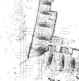
The following experiment has been made at the campus of Schloss Birlinghoven with Kurt3D. Fig. 3 (left) shows the scan point model of the first scans in top view, based on odometry only. The first part of the robot's run, i.e., driving on asphalt, contains a systematic drift error, but driving on lawn shows more stochastic characteristics. The right part shows the first 62 scans, covering a path length of about 240 m. The heuristic has been applied and the scans have been matched. The open loop is marked with a red rectangle.

At that point, the loop is detected and closed. More 3D scans have then been acquired and added to the map. Fig. 4 (left and right) shows the model with and without global relaxation to visualize its effects. The relaxation is able to align the scans correctly even without explicitly closing the loop. The best visible difference is marked by a red rectangle. The final map in Fig. 4 contains 77 3D scans, each consisting of approx. 100000 data points (275 $\times$ 361). Fig. 5 shows two detailed views, before and after loop closing. The bottom part of Fig. 4 displays an aerial view as ground truth for comparison. Table 1 compares distances measured in the photo and in the 3D scene. The lines in the photo have been measured in pixels, whereas real distances, i.e., the $ (x,z)$

-values of the points, have been used in the point model. Taking into account that pixel distances in mid-resolution non-calibrated aerial image induce some error in ground truth, the correspondence show that the point model at least approximates reality quite well.

**Figure 5:** Detailed view of the 3D model of Fig. 4. Left: Model before loop closing. Right: After loop closing, global relaxation and adding further 3D scans. Top: Top view. Bottom: Front view.
$\includegraphics[width=0.49\linewidth]{before_loop_closing_detail}$ $\includegraphics[width=0.49\linewidth]{after_loop_closing_detail}$ $\includegraphics[width=0.49\linewidth]{before_loop_closing_detail1}$ $\includegraphics[width=0.49\linewidth]{after_loop_closing_detail1}$ $\begin{picture}(10,10)(-95,-250)\thicklines {\color[rgb]{1,0,0}\put(0,0){\framebox (60,40){}} }% \end{picture}$ $\begin{picture}(10,10)(-255,-250)\thicklines {\color[rgb]{1,0,0}\put(0,0){\framebox (60,40){}} }% \end{picture}$ $\begin{picture}(10,10)(0,-80)\thicklines {\color[rgb]{1,0,0}\put(0,0){\framebox (65,45){}} }% \end{picture}$ $\begin{picture}(10,10)(-161,-80)\thicklines {\color[rgb]{1,0,0}\put(0,0){\framebox (65,45){}} }% \end{picture}$ $\includegraphics[width=45mm]{fahrradstaender}$

**Table 1:** Length ratio comparison of measured distances in the aerial photographs with distances in the point model as shown in Fig. 4.
1st line	2nd line	ratio in aerial views	ratio in point model	deviation
AB	BC	0.683	0.662	3.1%
AB	BD	0.645	0.670	3.8%
AC	CD	1.131	1.141	0.9%
CD	BD	1.088	1.082	0.5%

**Figure 6:** Detailed views of the resulting 3D model corresponding to robot locations of Fig. 1.
$\includegraphics[width=0.325\linewidth]{view6}$ $\includegraphics[width=0.325\linewidth]{view2}$ $\includegraphics[width=0.325\linewidth]{view3}$

Mapping would fail without first calculatingheuristic initial estimations for ICP scan matching, since ICP would likely converge into an incorrect minimum. The resulting 3D map would be some mixture of Fig. 3 (left) and Fig. 4 (right).

Fig. 6 shows three views of the final model. These model views correspond to the locations of Kurt3D in Fig. 1. An updated robot trajectory has been plotted into the scene. Thereby, we assign every 3D scan that part of the trajectory which leads from the previous scan pose to the current one. Since scan matching did align the scans, the trajectory initially has gaps after the alignment (see Fig. 7).

In addition we used the 3D scan matching algorithm in the context of RoboCup Rescue 2004. We were able to produce online 3D maps, even though we did not use closed loop detection and global relaxation. Some results are available at http://kos.informatik.uni-osnabrueck.de/download/Lisbon_RR/.