Next: Estimating Matching Quality
Up: Evaluating the Match
Previous: Evaluating the Match
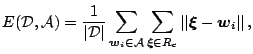
In addition to subsampling, goals of competitive object learning
are the minimization of the expected quantization error and
entropy maximization. A finite set of 3D scan points  is
subsambled to the set
is
subsambled to the set
 . Error minimization is done with respect to the following
function:
. Error minimization is done with respect to the following
function:
with the set  of samples and the Voronoi
set
of samples and the Voronoi
set
 of unit
  , i.e.,
 and
and
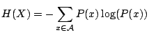
 . Entropy maximization guarantees inherent
robustness. The failure of reference vectors, i.e., missing 3D
points, affects only a limited fraction of the data. Interpreting
the generation of an input signal and the subsequent mapping onto
the nearest sample in as a random experiment which
assigns a value
. Entropy maximization guarantees inherent
robustness. The failure of reference vectors, i.e., missing 3D
points, affects only a limited fraction of the data. Interpreting
the generation of an input signal and the subsequent mapping onto
the nearest sample in as a random experiment which
assigns a value
 to the random variable
  , then
maximizing the entropy
, then
maximizing the entropy
is equivalent to equiprobable samples. The following neural gas
algorithm learns and subsamples 3D points clouds [7]:
- i.).
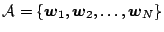
- Initialize the set
 to contain
  vectors, randomly
from the input set. Set
vectors, randomly
from the input set. Set  .
.
- ii.).
- Generate at random an input element
 , i.e., select a
point from
, i.e., select a
point from  .
.
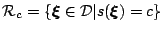
- iii.).
- Order all elements of according to their distance to
, i.e., find the sequence of indices
 such that
 is the reference
vector closest to ,
is the reference
vector closest to ,
 is the reference
vector second closest to , etc.,
is the reference
vector second closest to , etc.,
 ,
,
 is the reference vector such that
  vectors
  exists that are closer to than
.
exists that are closer to than
.
 denotes the number associated with
 .
.
- iv.).
- Adapt the reference vectors according to
with the following time dependencies:
- v.).
- Increase the time parameter
 .
.
The neural gas algorithms is used with the following parameters:
 ,
,
 ,
,
 ,
,
 ,
,
 max
max . Note that
max controls the run time. Fig.
. Note that
max controls the run time. Fig. ![[*]](file:/usr/share/latex2html/icons/crossref.png) shows 3D models of the database (top row) and subsampled versions
(bottom) with 250 points.
shows 3D models of the database (top row) and subsampled versions
(bottom) with 250 points.
Figure:
Top: 3D models (point clouds) of the database. Bottom:
sumbsampled models with 250 points.
|
|
Next: Estimating Matching Quality
Up: Evaluating the Match
Previous: Evaluating the Match
root
2005-05-03