


Next: Results and Conclusion
Up: Evaluating the Match
Previous: Competitive Object Learning
Given two registered point sets that contain an equal number of
points, e.g., 250 points derived under the premise of
minimization of the expected quantization error and entropy
maximization, the quality of a matching can be evaluated using
the following method: The distribution of shortest distances
 between the
  th and the
  th point (closest points)
after registering two models with a fixed (here: 250) number of
points show a typical structure (Fig.
th point (closest points)
after registering two models with a fixed (here: 250) number of
points show a typical structure (Fig. ![[*]](file:/usr/share/latex2html/icons/crossref.png) ).
Many distances are very small, i.e., less than 0.3 cm, and there
are also many larger distances, e.g., greater than 1 cm. To our
experience it is always easy to find a good threshold to separate
the two maximas. After dividing the set of distances
).
Many distances are very small, i.e., less than 0.3 cm, and there
are also many larger distances, e.g., greater than 1 cm. To our
experience it is always easy to find a good threshold to separate
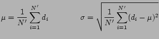
the two maximas. After dividing the set of distances  , the
algorithm computes the mean and the standard deviation of the
matching, i.e.,
, the
algorithm computes the mean and the standard deviation of the
matching, i.e.,
Based on these values one estimates the matching quality by
computing a measure  as a function of
  and
and  (we
have been using
(we
have been using
 ). Small values of
correspond to a high quality matching whereas increasing values
represent lower qualities.
). Small values of
correspond to a high quality matching whereas increasing values
represent lower qualities.
Figure:
A typical distribution of distances between closest
points after registering two models with a fixed (here: 250)
number of points.
|
|
Figure:
Examples of object detection and localization. From
Left to right: (1) Detection using single cascade of
classifiers. Green: detection in reflection image, yellow:
detection in depth image. (2) Detection using the combined
cascade. (3) Superimposed to the depth image is the matched 3D
model. (4) Detected object in the raw scanner data, i.e., point
representation.
|
|
Table:
Object name, number of stages used for
classification versus hit rate and the total number of false
alarms using the single and combined cascades. The test sets
consist of 89 images rendered from 20 3D scans. The average
processing time is also given, including the rendering,
classification, ray tracing, matching and evaluation
time.
|
object |
# stages |
detection rate (reflect. img. /
depth img.) |
false alarms (reflect. img. /
depth img.) |
average proc. time |
|
chair |
15 |
0.767 (0.867 / 0.767) |
12 (47 / 33)
|
1.9 sec |
| kurt robot |
19 |
0.912 (0.912 / 0.947) |
0 ( 5 / 7)
|
1.7 sec |
| volksbot robot |
13 |
0.844 (0.844 / 0.851) |
5 (42 / 23)
|
2.3 sec |
| human |
8 |
0.961 (0.963 / 0.961) |
1 (13 / 17)
|
1.6 sec |
Next: Results and Conclusion
Up: Evaluating the Match
Previous: Competitive Object Learning
root
2005-05-03
![\includegraphics[width=75mm]{barchart_color}](img123.png)
![\includegraphics[width=43mm,height=43mm]{kurt_009_singleCascades}](img124.png)
![\includegraphics[width=43mm,height=43mm]{kurt_009_combinedCascades}](img125.png)
![\includegraphics[width=43mm,height=43mm]{volksbot080_singleCascades}](img126.png)
![\includegraphics[width=43mm,height=43mm]{volksbot080_combinedCascades.eps}](img127.png)
![\includegraphics[width=43mm,height=43mm]{volksbot080_combinedCascades_with_model.eps}](img128.png)
![\includegraphics[width=43mm,height=43mm]{volksbot080_points_with_model.eps}](img129.png)
![\includegraphics[width=43mm,height=43mm]{human023_singleCascades}](img130.png)
![\includegraphics[width=43mm,height=43mm]{human023_combinedCascades}](img131.png)
![\includegraphics[width=43mm,height=43mm]{human023_combinedCascades_with_model}](img132.png)
![\includegraphics[width=43mm,height=43mm]{human023_points_with_model}](img133.png)
![\includegraphics[width=43mm,height=43mm]{volksbot014_singleCascades}](img134.png)
![\includegraphics[width=43mm,height=43mm]{volksbot014_combinedCascades}](img135.png)
![\includegraphics[width=43mm,height=43mm]{volksbot014_combinedCascades_with_model}](img136.png)
![\includegraphics[width=43mm,height=43mm]{volksbot014_points_with_model}](img137.png)